
The second step in transportation planning, known as trip distribution, focuses on connecting trip origins to destinations, and at worldtransport.net, we offer insights into this crucial phase of urban travel demand forecasting. By understanding how trips are distributed, we can optimize transportation systems, reduce congestion, and improve accessibility for everyone.
1. Understanding Trip Distribution in Transportation Planning
Trip distribution is the pivotal second step in the Four-Step Model (FSM) of transportation planning. After the initial stage of trip generation, which quantifies the number of trips originating from and destined for specific zones, trip distribution focuses on connecting these origins and destinations. This process determines the flow of trips between each pair of zones within the study area, transforming the aggregated trip numbers into a detailed Origin-Destination (O-D) matrix. These matrices, also known as trip tables, are essential for understanding travel patterns and are a fundamental input for subsequent stages of transportation planning.
According to the National Highway Institute (NHI), trip distribution plays a critical role in answering the question: What portion of trips produced in or attracted to a zone would go to each of the other zones? This step considers the attractiveness of each zone and the impedance, such as travel time or cost, between zones. The most commonly used method for estimating trip distribution is the gravity model, although growth factor models and intervening opportunities models are also utilized.
Trip distribution is crucial because it bridges the gap between trip generation and the later steps of mode choice and route assignment. By accurately modeling how trips are distributed, planners can better predict traffic volumes on specific roadways, assess the impact of new developments on the transportation network, and evaluate the effectiveness of different transportation policies and investments.
1.1. Key Factors Influencing Trip Distribution
Several factors influence how trips are distributed between zones, including:
- Attractiveness of Zones: Zones with more employment opportunities, retail services, or recreational facilities tend to attract more trips. The uniqueness of a zone’s offerings can also significantly increase its attractiveness, regardless of distance.
- Spatial Separation (Distance): The distance between two zones acts as an impedance, with longer distances generally resulting in fewer trips between them. People are less likely to travel long distances for everyday activities, so zones that are closer together tend to have higher trip volumes.
- Proximity to Other Services: Zones located near other desirable services or amenities tend to attract more trips. This clustering effect can increase the overall attractiveness of a zone and make it a more popular destination.
- Urban vs. Rural Classification: The attraction rate for a zone can vary based on whether it is located in an urban or rural area. Urban areas typically have higher densities of activities and services, leading to higher trip attraction rates.
- Emissivity Factors: The origin’s emissivity, often represented by population, employment, or income, also plays a crucial role. Zones with higher populations or employment levels tend to generate more trips.
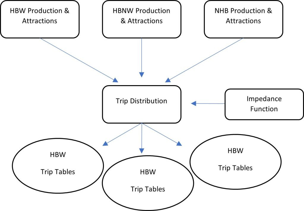 Trip attractions and productions resulting in a matrix for each trip purpose.
1.2. Essential Inputs for Trip Distribution
Before calculating trip distribution, several foundational components must be considered, independent of the FSM framework or the methods used for estimation. These components serve as inputs for estimating trip distribution and are critical for accurate modeling. The main inputs include:
- Trip Productions and Attractions (P-A Trips): The output from the trip generation step, which estimates the number of trips originating from and destined for each zone.
- Interzonal Transportation Costs: Measures of the impedance or difficulty of traveling between zones, such as travel time, distance, or cost.
- Socio-Economic Factors: Data on population, employment, income, and other socio-economic characteristics of each zone, which can influence travel behavior.
2. Delving into the Gravity Model for Trip Distribution
The gravity model is the most commonly used method for estimating trip distribution due to its simplicity, accuracy, and ability to incorporate various factors such as population, employment, socio-demographics, and transportation systems. Almost all U.S. Departments of Transportation (DOTs) utilize gravity models for transportation planning.
The gravity model is built on the concept that the number of trips between two zones is directly proportional to the attractiveness of the destination zone and inversely proportional to a function of cost, such as travel time or trip cost. This model is inspired by Newton’s Law of Gravity, which states that the attraction between two bodies is related to their mass (positive attraction) and the distance between them (negative attraction).
According to the Transportation Planning Handbook by Michael D. Meyer, numerous studies confirm that people value travel time differently based on the purpose of the trip, such as work trips versus recreational trips. Therefore, it is rational to compute the gravity model for each trip purpose using different impedance factors.
2.1. The Fundamental Equation of Trip Distribution
The gravity model can be represented in several different ways. The fundamental equation of trip distribution is:
Tij = Pi * (Aj * FFij * Kij) / Σ(Aj * FFij * Kij)
Where:
- Tij = Number of trips between zone i and zone j
- Pi = Total number of trips produced in zone i
- Aj = Number of trips attracted to zone j
- FFij = Friction factor (travel impedance) between i and j
- Kij = Socio-economic adjustment factor for interchange ij
2.2. Breaking Down the Components of the Gravity Model
Each component of the gravity model plays a crucial role in determining the trip distribution pattern:
- Trip Productions (Pi): The total number of trips originating from zone i, determined during the trip generation process.
- Trip Attractions (Aj): The total number of trips destined for zone j, also determined during the trip generation process.
- Friction Factor (FFij): A value representing the impedance or difficulty of traveling between zone i and zone j. This factor captures the spatial separation between zones and is often represented as travel time or cost.
- Socio-Economic Adjustment Factor (Kij): A factor that adjusts for socio-economic differences between zones i and j that may influence travel behavior. This factor accounts for variations in income, auto ownership, and other factors that can affect trip-making patterns.
According to research from the Center for Transportation Research at the University of Illinois Chicago, in July 2025, The Pi and Aj values are determined through the trip generation process. The sum of all productions and attractions should be equal. Numerous studies confirm that people value travel time differently based on the purpose of the trip (like work trips vs. recreational trips). Therefore, it is rational to compute the gravity model for each trip purpose using different impedance factors.
2.3. Understanding the Impedance Factor
The impedance factor, also known as the friction factor, is a critical element in the gravity model. It reflects the difficulty of traveling between two zones and is influenced by factors such as travel time, distance, and cost. The friction factor is higher when accessibility between two zones is easy and is zero if no individual is willing to travel between two zones.
Friction factors can be estimated using different measures, including:
- Travel Time: A simple measure of friction is the travel time between the zones.
- Exponential Formula: Another method is adopting an exponential formula with the 1/exp (m × Tij) friction factor, where m is the average travel time calculated using empirical data.
- Gamma Distribution: Uses scaling factors to estimate distribution.
The impedance factor reflects the difficulty of traveling between two zones. The friction factor is higher when accessibility between two zones is easy and is zero if no individual is willing to travel between two zones. The friction factor estimation process also involves a calibration step. For calibration, trip generation and attraction values are distributed between O-D pairs using the gravity model. Next, the number of trips is compared with a particular amount of time to the results of the O-D survey (observed data). If the numbers do not match, calibration adjusts for the friction factor. When using travel time as the measure of impedance, the relationship between the friction factor and time is represented as t-1, t–2, e– t.
The figure below (Figure 11.2) shows the function of the friction factor appropriate to the time and for different trip purposes. As the figure shows, there is a direct relationship between friction factor and travel time. According to this figure, for each trip purpose, there is a perception about the length or impedance of trip. Beyond certain length, friction factor approaches zero, meaning a high level of disutility of the trip and this threshold is different for each trip purpose.
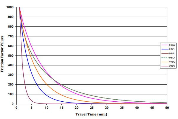 This figure shows the curve of impedance function calibrated for each trip purpose.
2.4. Incorporating Socio-Economic Factors with the K-Factor
Travel demand modeling is influenced by various socio-economic factors that affect travel behavior and demand for different purposes. These factors include income, auto ownership, availability of multimodal transportation systems, age, and job type. To account for these factors, the K-Factor method was developed and integrated into the gravity model.
The K-factor is determined and plugged into the gravity formula to accommodate such differences. Calibration of K values is determined by comparing the estimated results and observed data for the base year. The K numeric value will be above one (>1) if the socio-economic factors contribute to more travel and less than one (<1) if they contribute to less travel.
Figure 11.3 shows the number of trips by age for work, shopping, family, and social purposes for three years. This data can be used to inform the K-factor and adjust the model accordingly.
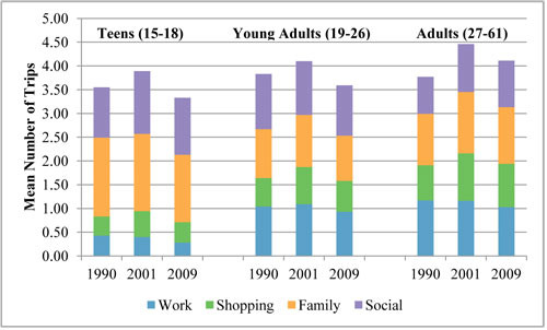 number of trips by age for work, shopping, family and social for three years.
3. Growth Factor Model: An Alternative Approach
The growth factor model is an alternative method for estimating trip distribution, particularly useful when friction factor and K-factor data are unavailable or unsatisfactorily calibrated. This model predicts future trip distributions based on changes in land-use data, socioeconomic data, or other system-wide changes.
However, growth factor models are limited if an observed O-D table is unavailable, as they rely on historical trends and data. Additionally, similar to the trip generation step, growth factor models cannot easily incorporate updated travel time, which can significantly affect travel patterns.
3.1. The Fratar Method
One of the most common mathematical formulas of the growth factor model is the Fratar method. This method estimates the future distribution of trips from one zone by multiplying the present distribution by the growth factor of the destination zone between the present and the forecasting year. The formula to calculate future trip values is:
Tij = (ti * Gi) * (tij * Gj) / Σ(tix * Gx)
Where:
- Tij = Number of trips estimated from zone to zone
- ti = Present trip generation in zone
- Gx = Growth factor of zone
- Ti = Future trip generation in zone
- tix = Number of trips between zone and other zones
- tij = Present trips between zone and zone
- Gj = Growth factor of zone
3.2. Practical Applications of Growth Factor Models
Growth factor models are particularly useful in situations where detailed data on travel impedance and socio-economic factors are limited. They can provide a quick and straightforward way to estimate future trip distributions based on overall growth trends.
However, it’s essential to recognize the limitations of these models. They assume that existing travel patterns will remain relatively stable and may not accurately capture the impact of significant changes in the transportation system or land use.
4. Model Calibration and Validation: Ensuring Accuracy
Model validation is an integral part of all simulation and modeling procedures. One of the most essential steps in FSM modeling is developing a procedure to calibrate its final outputs (predictions) with actual and observed data. To do this, model parameters are adjusted so that the observed data and estimations have fewer mismatches. After such adjustments, the model with calibrated parameters can help in simulation and future scenario analyses.
After completing the trip distribution step, it is important to compare model calibration and adjustment results in each category (i.e., by trip purpose) with recorded real-world trips from the O-D survey. If the two values are not identical, model parameters, like FF or K-factors, are reassigned and re-run the gravity model. The process continues until the observed data and estimations are very close (ratio between 0.9 and 1.1).
5. Real-World Examples and Case Studies
To illustrate the application of trip distribution methods, let’s consider a few real-world examples and case studies.
5.1. Hypothetical Area Scenario
In a hypothetical area, we are interested in determining the number of trips attracted by three different shopping malls at various distances from a university campus that generates about 2,000 trips per day. The number of trips generated by the campus and the total number of trips attracted for each zone are presented in Figure 11.4.
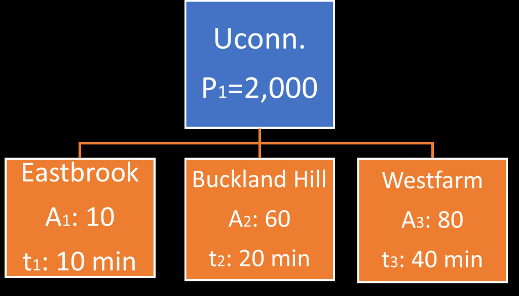 This figure shows the trip generator and the three possible destination with their travel time.
By applying the gravity model and considering factors such as travel time and attractiveness of each shopping mall, we can estimate the number of trips attracted from the campus to each zone. The final results, as shown in Figure 11.5, provide valuable insights into the distribution of trips and can inform transportation planning decisions.
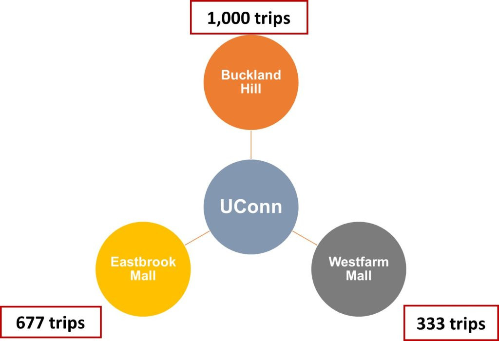 This figure shows the results of example 3 graphically.
5.2. Lincoln Travel Demand Model
The Lincoln Travel Demand Model, developed by Lima & Associates, provides a real-world example of how trip distribution is applied in urban transportation planning. This model uses the gravity model to estimate trip distribution in the Lincoln, Nebraska metropolitan area.
The model considers various factors, including travel time, socio-economic data, and land use patterns, to accurately predict travel patterns. The friction factor distribution by trip purpose, as shown in Figure 11.2, is a key component of the model.
6. Modern Advancements and Innovations in Trip Distribution
While traditional methods like the gravity model and growth factor models remain widely used, modern advancements and innovations are enhancing trip distribution techniques. These include:
- Dynamic Modeling: Concurrent mode and destination choice models that allow for more realistic representation of travel behavior.
- Micro-simulation: Detailed simulation models that can capture the complex interactions of individual travelers.
- Agent-Based Models: Models that simulate the behavior of individual agents (travelers) and their interactions with the transportation system.
- Machine Learning: Newer methods that can identify patterns and predict travel behavior based on large datasets.
These advancements, combined with the collection of real-time data and increased computational capacity, are opening new prospects in travel demand modeling and trip distribution studies.
7. Conclusion: The Path Forward in Transportation Planning
Trip distribution is a critical step in transportation planning that bridges the gap between trip generation and subsequent stages like mode choice and route assignment. By understanding how trips are distributed, planners can make informed decisions about transportation investments, policies, and strategies.
While traditional methods like the gravity model and growth factor models remain valuable, modern advancements and innovations are enhancing trip distribution techniques. These include dynamic modeling, micro-simulation, agent-based models, and machine learning.
At worldtransport.net, we provide comprehensive information and insights into the latest trends and best practices in transportation planning. We encourage you to explore our website to learn more about trip distribution and other essential topics in the field.
For further information or assistance with your transportation planning needs, please contact us:
- Address: 200 E Randolph St, Chicago, IL 60601, United States
- Phone: +1 (312) 742-2000
- Website: worldtransport.net
8. Frequently Asked Questions (FAQ)
- What is trip distribution in transportation planning?
Trip distribution is the second step in the Four-Step Model (FSM) of transportation planning, focusing on connecting trip origins to destinations. It transforms the aggregated trip numbers from the trip generation stage into a detailed Origin-Destination (O-D) matrix, essential for understanding travel patterns. - Why is trip distribution important?
Trip distribution is crucial because it bridges the gap between trip generation and the later steps of mode choice and route assignment. By accurately modeling how trips are distributed, planners can better predict traffic volumes, assess the impact of new developments, and evaluate the effectiveness of different transportation policies. - What factors influence trip distribution?
Several factors influence trip distribution, including the attractiveness of zones (employment, retail, recreation), spatial separation (distance), proximity to other services, urban vs. rural classification, and emissivity factors (population, employment, income). - What is the gravity model?
The gravity model is the most commonly used method for estimating trip distribution. It’s built on the concept that the number of trips between two zones is directly proportional to the attractiveness of the destination zone and inversely proportional to a function of cost, such as travel time or trip cost. - What is the friction factor in the gravity model?
The friction factor, also known as the impedance factor, is a value representing the difficulty of traveling between two zones. It reflects the spatial separation between zones and is often represented as travel time, distance, or cost. - What is the K-factor in the gravity model?
The K-factor is a socio-economic adjustment factor that accounts for socio-economic differences between zones that may influence travel behavior, such as income, auto ownership, and other factors. - What is the growth factor model?
The growth factor model is an alternative method for estimating trip distribution, particularly useful when friction factor and K-factor data are unavailable. It predicts future trip distributions based on changes in land-use data, socioeconomic data, or other system-wide changes. - What is the Fratar method?
The Fratar method is one of the most common mathematical formulas of the growth factor model. It estimates the future distribution of trips from one zone by multiplying the present distribution by the growth factor of the destination zone between the present and the forecasting year. - Why is model calibration and validation important?
Model calibration and validation are essential to ensure the accuracy of trip distribution models. Model parameters are adjusted so that the observed data and estimations have fewer mismatches, allowing for more reliable simulation and future scenario analyses. - What are some modern advancements in trip distribution?
Modern advancements in trip distribution include dynamic modeling, micro-simulation, agent-based models, and machine learning. These techniques, combined with real-time data collection and increased computational capacity, are opening new prospects in travel demand modeling.