
Trip distribution in transportation planning is a crucial step that helps us understand and predict travel patterns. At worldtransport.net, we break down this complex process, explaining how it connects origins and destinations, considering factors like travel time and cost. This information is vital for effective transportation solutions, and we’re here to guide you through it. Explore worldtransport.net for in-depth analysis, trends, and solutions that are shaping the future of transportation.
1. Understanding Trip Distribution in Transportation Planning
Trip distribution is a core component of the four-step travel demand model (FSM), which is used to forecast travel demand in a specific area. So, what exactly is trip distribution in transportation planning?
Trip distribution determines the number of trips between different zones, turning trip generation data into an origin-destination matrix. Following trip generation, the crucial second step of the Four-Step Model (FSM) involves calculating the number of trips between each pair of zones. This process is known as trip distribution. These outputs are commonly referred to as Origin-Destination pairs (O-D pairs or Tij), representing the number of trips between Zone i (origin) and Zone j (destination) (Levine, 2010). Essentially, trip distribution transforms the results of the first FSM step into a detailed matrix showing origins and destinations within Traffic Analysis Zones (TAZs), while also considering travel impedance factors such as travel time or cost for each O-D pair.
Trip distribution answers the central question: “What portion of trips produced in or attracted to a zone will go to each of the other zones?” Common methods to estimate trip distribution include growth factor models, the intervening opportunities model, and the gravity model.
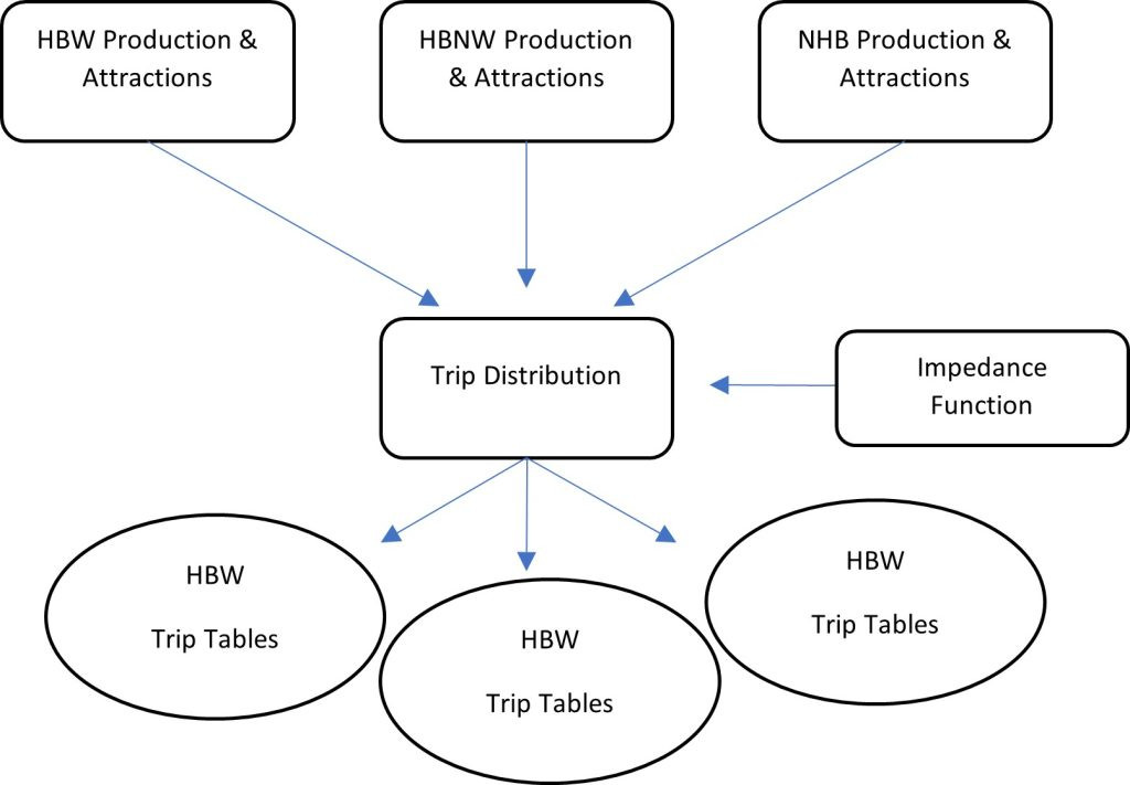 trip attractions and productions resulting in a matrix for each trip purpose
Several foundational components must be considered before calculating trip distribution, independent of the FSM framework or the methods used for trip distribution estimation. Trip distribution is the second step of the FSM, where trip productions are allocated to all other zones, yielding a matrix that displays the number of both intrazonal and interzonal trips in a single table (Lincoln MPO, 2011).
2. Key Factors Influencing Trip Distribution
Several factors influence the number of trips between zones. These can be broadly categorized into attractiveness factors and emissivity factors.
2.1. Attractiveness Factors
What makes a zone attractive to travelers?
A zone’s attractiveness is determined by its uniqueness, distance from other zones, proximity to services, and its urban or rural classification. The attractiveness of a zone is influenced by several factors (Cesario, 1973):
- Uniqueness: Unique services or employment centers attract more trips, regardless of distance.
- Distance: Greater spatial separation between zones reduces trip distribution.
- Closeness to other services: Proximity to desirable services increases trip attraction within an urban area.
- Urban or rural area: Attraction rates differ based on urban or rural classification, while controlling for other factors.
2.2. Emissivity Factors
What determines how many trips originate from a zone?
A zone’s emissivity, usually represented by population, employment, or income, affects the number of trips it produces. The origin zone also has an emissivity factor, typically represented by population, employment, or income (Cesario, 1973). With a general understanding of the factors affecting trip distribution from origin and destination, we can now explore the methodology.
3. Common Methods for Trip Distribution Estimation
Several methods can be used to estimate trip distribution. Here are some of the most common approaches.
3.1. Gravity Model
How does the gravity model help in estimating trip distribution?
The gravity model, inspired by Newton’s Law of Gravity, is the most common method, relating trip numbers to the attractiveness of destination zones and the impedance of travel. The gravity model is the most common method used to estimate trip distribution due to its ease of understanding and accuracy, accommodating various factors such as population, employment, socio-demographics, and transportation systems. Almost all U.S. Departments of Transportation (DOTs) use gravity models. In contrast, the Growth Factor Model requires additional data about trip distribution in the base year and an estimate of the number of future trips in each zone, which is only sometimes available (Meyer, 2016).
The Gravity Model is based on the number of trips made between two zones, directly linked to the total number of attractions in the destination zone and inversely proportional to a function of cost, such as travel time or trip cost (Council, 2006). The formula gets its name from Newton’s Law of Gravity, which states that the attractiveness between two bodies is related to their mass (positive attraction) and the distance between them (negative attraction) (Verlinde, 2011). In transportation modeling, the two main factors are trip production and attraction, along with the time duration of travel or the cost of travel.
Equation below shows the fundamental equation of trip distribution:
Trips between TAZ1 and TAZ2=Trips prodduced in TAZ1*(Attractiveness of TAZ2 /Attractiveness of all TAZs
As equation (1) shows, the total trips between zones are equal to the products of the trips produced in a zone, a ratio of the attractiveness of the destination zone, and the total attractiveness of all zones.
The mathematical format of the gravity model can be seen in equation below:
Where:
- Tij = number of trips that are produced in zone i and attracted to zone j
- Pi = total number of trips produced in zone i
- Aj = number of trips attracted to zone j
- Fij = a value which is an inverse function of travel time
- Kij = socioeconomic adjustment factor for interchange ij
The Pi and Aj values are determined through the trip generation process (refer to Chapter 10), and the sum of all productions and attractions should be equal (PE, 2017). Numerous studies confirm that people value travel time differently based on the purpose of the trip (like work trips vs. recreational trips) (Hansen, 1962; Allen, 1984; Thill & Kim, 2005). Therefore, it is rational to compute the gravity model for each trip purpose using different impedance factors (Meyer, 2016).
3.1.1. Impedance Factor in Gravity Model
What role does the impedance factor play in the gravity model?
The impedance factor, or friction factor, represents the difficulty of traveling between two zones, often measured as travel time or cost. The impedance factor (aka friction factor) is a value that varies for different trip purposes because, with the FSM model, the assumption is that travel behavior depends on trip purpose. Impedance captures the spatial separation between two zones, represented as travel time or cost.
Friction factors (FF) can be estimated using different measure, as follows:
- A simple measure of friction is the travel time between the zones.
- Another method is adopting an exponential formula with the 1/exp (m × Tij) friction factor, where m is the average travel time calculated using empirical data.
- Gamma distribution uses scaling factors to estimate distribution (Cambridge Systematics, 2010; Meyer, 2016).
The friction factor is higher when accessibility between two zones is easy and is zero if no individual is willing to travel between two zones.
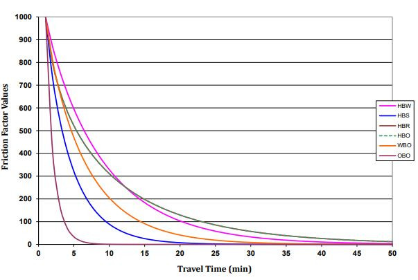 This figure shows the curve of impedance function calibrated for each trip purpose
There is also a calibration step in the friction factor estimation process. For calibration, trip generation and attraction values are distributed between O-D pairs using the gravity model. Next, the number of trips is compared with a particular amount of time to the results of the O-D survey (observed data). If the numbers do not match, calibration adjusts for the friction factor. When using travel time as the measure of impedance, the relationship between the friction factor and time in the is represented as t-1, t–2, e– t (Ashford & Covault, 1969).
3.1.2. K-Factor in Gravity Model
What does the K-factor represent in the gravity model?
The K-factor adjusts interzonal trips to account for socio-economic factors influencing travel behavior, such as income, auto ownership, and job type. Travel demand modeling is influenced by various socio-economic factors that affect travel behavior and demand for different purposes. Chapter 10 highlights the most significant factors in travel demand modeling: income, auto ownership, availability of multimodal transportation systems, age, and job type (Pan et al., 2020). Therefore, the K-Factor method was developed and plugged into the gravity model to represent variation in socio-economic factors and adjust interzonal trips accordingly. For example, a blue-collar employee working in a low-income suburb may exhibit different travel behaviors (in terms of mode choice and frequency of travel) compared to a white-collar employee working in the central city with a higher income. The K-factor is determined and plugged into the gravity formula to accommodate such differences.
3.2. Growth Factor Model
How does the Growth Factor Model predict future trip distributions?
The Growth Factor Model predicts future trip distributions based on changes in land use and socio-economic data, using historical trends when other data is unavailable. After successfully calibrating and validating the data we have estimated, we can also apply the gravity model to forecast future travel behavior or travel patterns in our study area. Future trip distributions can be predicted by using the change in land-use data, socioeconomic data, or any other changes in the whole system. We can calculate trip distribution from the O-D table for either base or forecasting year when the friction factor and K-factor data are unavailable or unsatisfactorily calibrated. Depending on historical trends and data, growth factor models are limited if an observed O-D table is unavailable. Similar to the trip generation step, growth factor models cannot incorporate updated travel time as the change in travel time between zones can highly affect travel patterns (Qsim, 2016).
3.2.1. Fratar Method
What is the Fratar method and how is it used in the Growth Factor Model?
The Fratar method, a common mathematical formula of the growth factor model, calculates future trip distribution based on the present distribution multiplied by the growth factor of the destination zone. One of the most common mathematical formulas of the growth factor model is the Fratar method, shown in the following equation. Through his method, the future distribution of trips from one zone is equal to the present distribution multiplied by the growth factor of the destination zone between now and the forecasting year (Heanue & Pyers, 1966).
Where:
- Tij =number of trips estimated from zone to zone
- ti =present trip generation in zone
- Gx =growth factor of zone
- Ti =future trip generation in zone
- tix =number of trips between zone and other zones
- tij =present trips between zone and zone
- Gj =growth factor of zone
4. Examples of Trip Distribution Calculations
Let’s dive into some examples to illustrate how trip distribution is calculated using different methods.
4.1. Example 1: Gravity Model Calculation
How is trip distribution calculated using the gravity model in a simplified scenario?
In a three-zone area, trip distribution is calculated using trip generation data, travel time, and friction factors to estimate the number of trips between each zone. Consider a small area with three zones (TAZs). The gravity model is used to calculate trip distribution between the three zones. The trip generation and attraction table from step one of the FSM model is the input data. Tables 11.1, 11.2, and 11.3 represent the trip generated and attracted for each zone, travel time between each pair of zones, and friction factor derived from the travel time.
Table 11.1 Trip Generation Results.
| TAZ | 1 | 2 | 3 | total |
|---|---|---|---|---|
| Trips Productions | 220 | 245 | 305 | 770 |
| Trip Attractions | 210 | 270 | 350 | 770 |
Table 11.2 Travel Time Matrix.
| TAZ | 1 | 2 | 3 |
|---|---|---|---|
| 1 | 6 | 4 | 2 |
| 2 | 4 | 5 | 4 |
| 3 | 2 | 4 | 5 |
Table 11.3 Travel time and Friction Factor.
| Travel Time | FF |
|---|---|
| 1 | 82 |
| 2 | 52 |
| 3 | 50 |
| 4 | 41 |
| 5 | 35 |
| 6 | 26 |
| 7 | 20 |
| 8 | 13 |
| 9 | 9 |
| 10 | 5 |
Using this information, we can start the calculation process. First, we have to estimate the attractiveness of each zone using the equation (1)
For example, for zone 1 we have:
Attractiveness1= 210*26=5460
Attractiveness2= 210*35=7350
Attractiveness3= 350*35=12250
Now, we use the pivotal formula of the gravity model (equation 2). Accordingly, we have (K-factor set to 1):
=35
=70
=115
=65
=65
=71
=108
=97
=98
=109
The result of the calculation is summarized in Table 11.4:
Table 11.4 Trip distribution results.
| TAZ | 1 | 2 | 3 | Calculated | Observed |
|---|---|---|---|---|---|
| 1 | 35 | 70 | 115 | 220 | 200 |
| 2 | 65 | 71 | 108 | 244 | 248 |
| 3 | 97 | 98 | 109 | 304 | 320 |
| Calculated | 197 | 239 | 332 | 768 | 768 |
| Observed | 210 | 288 | 270 | 768 |
4.2. Example 2: Fratar Method Application
How is the Fratar method applied to estimate future trip distributions in a four-zone area?
The Fratar method is applied using current trip distributions and growth rates for each zone to calculate future trip numbers between zones, with iterations to align estimated and actual trip generations. The case study area of this example consists of four TAZs. Table 11.5 shows the current trip distributions. Assuming the growth rate for each TAZ is shown in Table 11.6, the next step is to calculate the number of trips between each two TAZs in the future year.
Table 11.5 Current trip distribution.
| TAZ | A | B | C |
|---|---|---|---|
| A | n/a | 300 | 200 |
| B | 150 | n/a | 100 |
| C | 100 | 200 | n/a |
| Total | 250 | 500 | 300 |
Table 11.6 Current trip distribution.
| TAZ | Total Generation | Growth Factor | Total Generation for Forecasting Year |
|---|---|---|---|
| A | 250 | 1.3 | 325 |
| B | 500 | 1.5 | 750 |
| C | 300 | 1.1 | 330 |
To solve this problem, apply the Fratar Method using the required two estimates for each pair. These estimates should be averaged; the resulting value will be the final Tij. Based on the formula, calculations are as follows:
Based on the calculations, the first iteration of the method will yield the following table:
Table 11.7 Estimated trip distribution using Fratar formula.
| TAZ | A | B | C | Estimated Total Generation | Actual Total Generations |
|---|---|---|---|---|---|
| A | n/a | 349 | 103 | 452 | 490 |
| B | 349 | n/a | 285 | 634 | 600 |
| C | 103 | 285 | n/a | 388 | 420 |
| Total | 452 | 500 | 300 |
4.3. Example 3: Trip Distribution Among Shopping Malls
How is trip distribution determined among multiple shopping malls based on travel time and attractiveness?
The number of trips attracted by three different shopping malls at varying distances from a university campus is determined using travel time, friction factors, and the gravity model. In a hypothetical area, we are interested in determining the number of trips attracted by three different shopping malls at various distances from a university campus that generates about 2,000 trips per day.
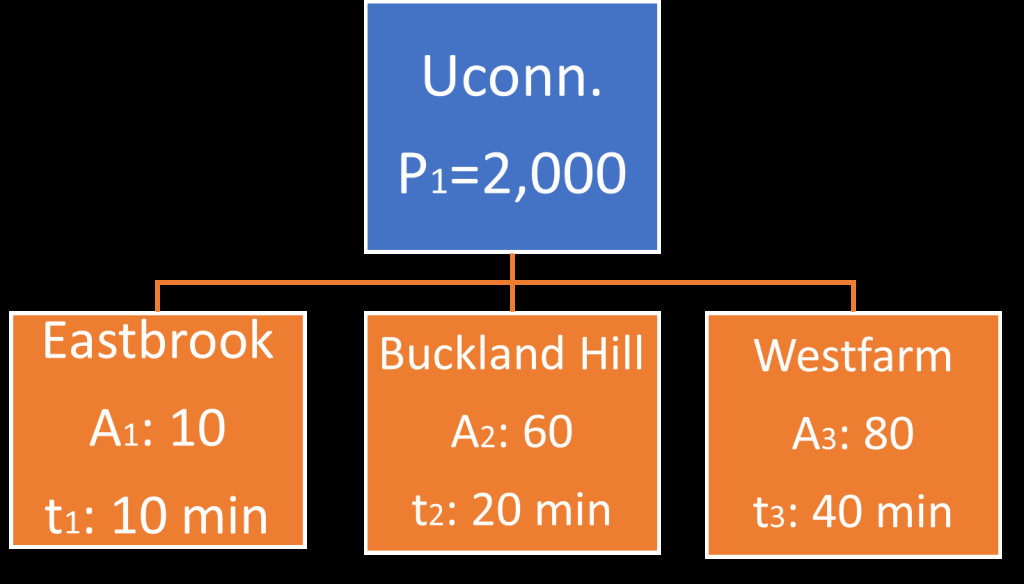 This figure shows the trip generator and the three possible destination with their travel time
Figure 11.4 Schematic Orientation of Trip Generation zone and Trip Attracting Zones.
As the first step, we need to calculate the friction factor for each pair of zones based on travel time (t). Given is the following formula with which we calculate friction factor:
Next, using the friction factor, we use the gravity model to calculate the relative attractiveness of each zone. In Table 11.8 , you can see how calculations are being carried out for each zone.
Table 11.8 Calculation of trip distribution (Friction Factor and Relative Attractiveness).
| J | Aj | t1j | F1j=tij^(-2) | Aj*F1j |
|---|---|---|---|---|
| 1 | 10 | 10 | 1/100=0.01 | 0.1 |
| 2 | 60 | 20 | 1/400=0.0025 | 0.15 |
| 3 | 80 | 40 | 1/1600=0.000625 | 0.05 |
| Total | 0.3 |
Table 11.9 Calculation of Final trip distribution.
| J | Aj*F1j | P1j= | T1j= P1*p1j |
|---|---|---|---|
| 1 (Eastbrook Mall) | 0.1 | 0.1/0.30=0.333 | 2,000*0.33=667 |
| 2 (Buckland Hill) | 0.15 | 0.15/0.3=0.5 | 2,000*0.5=1,000 |
| 3 (Westfarm Mall) | 0.05 | 0.05/0.3=0.167 | 2,000*0.167=333 |
| Total | 0.3 | 1 | 2000 |
Next, with having relative attractiveness of each zone (or probability of attracting trips), we plug in the trip generation rate for the campus (6,000) to finally estimate the number of trips attracted from the campus to each zone. Figure 11.5 shows the final results.
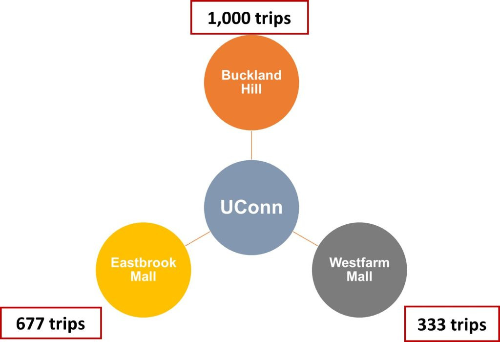 This figure shows the results of example 3 graphically
5. Model Calibration and Validation
Why is model calibration and validation important in trip distribution?
Model calibration and validation ensure that the trip distribution model’s predictions align with real-world data, enhancing the model’s reliability for future scenario analyses. Model validation is an integral part of all simulation and modeling procedures. One of the most essential steps in FSM modeling is developing a procedure to calibrate its final outputs (predictions) with actual and observed data. To do this, model parameters are adjusted so that the observed data and estimations have fewer mismatches (Meyer, 2016). After such adjustments, the model with calibrated parameters can help in simulation and future scenario analyses.
After completing the trip distribution step, it is important to compare model calibration and adjustment results in each category (i.e., by trip purpose) with recorded real-world trips from the O-D survey.
If the two values are not identical, model parameters, like FF or K-factors, are reassigned and re-run the gravity model. The process continues until the observed data and estimations are very close (ratio between 0.9 and 1.1).
5.1. Example 4: Calibration Process
How is the calibration process carried out to align model predictions with observed data?
The calibration process involves adjusting model parameters like friction factors and K-factors through multiple iterations until the model’s outputs closely match observed trip data. This example demonstrates the calibration process. The first step is to identify the model’s inputs, which are the outcomes of the trip generation process. The following tables show the results obtained from surveys and actual trip data, as well as the travel time between each pair of zones (represented by the friction factor (FF)) and the socioeconomic conditions (Tables 11.10, 11.11, and 11.12 ). The column with the heading “A’ “in Table 11.11 represents observed generated trips.
Table 11.10 Travel Time Matrix.
| Travel Time Matrix | blank cell | ||
|---|---|---|---|
| Zone | 1 | 2 | 3 |
| 1 | 1 | 6 | 11 |
| 2 | 7 | 3 | 12 |
| 3 | 15 | 13 | 4 |
Table 11.11 Trip Generation Results.
| Outcomes of trip generation | blank cell | blank cell | blank cell |
|---|---|---|---|
| Zone | P | A | A’ |
| 1 | 550 | 440 | 400 |
| 2 | 600 | 682 | 620 |
| 3 | 380 | 561 | 510 |
| 1530 | 1683 | 1530 |
Table 11.12 FF Matrix.
| Friction Factors | blank cell | ||
|---|---|---|---|
| Zone | 1 | 2 | 3 |
| 1 | 0.876 | 1.554 | 0.77 |
| 2 | 1.554 | 0.876 | 0.77 |
| 3 | 0.77 | 0.77 | 0.876 |
Table 11.13 K-factor Matrix.
| K Factors | blank cell | blank cell | blank cell |
|---|---|---|---|
| Zone | 1 | 2 | 3 |
| 1 | 1.04 | 1.15 | 0.66 |
| 2 | 1.06 | 0.79 | 1.14 |
| 3 | 0.76 | 0.94 | 1.16 |
To estimate the number of trips between each pair of zones, we use the gravity formula and input the necessary data. Table 11.14 shows the results of trip distribution for each pair of zones. However, the total number of trips attracted from our calculations is different from observed data.
Table 11.14 Trip Distribution Results.
| Zone | 1 | 2 | 3 | produced |
|---|---|---|---|---|
| 1 | 116 | 352 | 82 | 550 |
| 2 | 257 | 168 | 175 | 600 |
| 3 | 74 | 142 | 164 | 380 |
| attracted | 447 | 662 | 421 | |
| 400 | 620 | 510 |
In the next step, we apply the calibration methods in order to make our final results more accurate.
Table 11.15 First iteration by row (correct for generation).
| Zone | 1 | 2 | 3 | blank cell |
|---|---|---|---|---|
| 1 | 104 | 330 | 100 | 533 |
| 2 | 230 | 157 | 212 | 599 |
| 3 | 66 | 133 | 199 | 398 |
| 400 | 620 | 510 |
In the first iteration of calibration, we have to generate a value called column factor, which is the result of dividing actual data attraction by estimated attractions. Then we apply this number for each pair in the same column. In Table 11.15, we can observe that the sum of attractions is now the same as the actual data, but the sum of generation amounts is now different from actual data generation. In this step, we perform another iteration, the same as the first iteration but instead of column factor, we plug in row factor value, which is the result of dividing actual data trip generation by estimated generation.
Table 11.16 Second Iteration by Column (Correct for attraction).
| Zone | 1 | 2 | 3 | blank cell |
|---|---|---|---|---|
| 1 | 107 | 340 | 103 | 550 |
| 2 | 231 | 157 | 212 | 600 |
| 3 | 63 | 127 | 190 | 380 |
| 401 | 625 | 505 | ||
| Col. F | 0.998364 | 0.992373 | 1.010743 |
A third iteration is needed because the sum of attraction is still different from the actual data, and we must generate another column factor. The results are shown in Table 11.17.
Table 11.17 Third iteration by column (correct for attraction).
| Zone | 1 | 2 | 3 | blank cell |
|---|---|---|---|---|
| 1 | 107 | 338 | 104 | 548 |
| 2 | 230 | 156 | 214 | 601 |
| 3 | 63 | 126 | 192 | 381 |
| 400 | 620 | 510 |
6. Conclusion: The Importance of Trip Distribution
Trip distribution is a vital step in transportation planning, linking trip generation with mode choice and route assignment. While traditional models have limitations, newer methods like machine learning and real-time data collection enhance travel demand modeling and trip distribution studies.
Are you facing challenges in understanding transportation trends or finding effective solutions? Visit worldtransport.net for comprehensive insights and innovative strategies. Our team is ready to provide the support and expertise you need to navigate the complexities of the transportation industry. Contact us today and let us help you drive your projects forward.
7. FAQ: Understanding Trip Distribution
7.1. What factors affect the attractiveness of zones in trip distribution?
A zone’s attractiveness in trip distribution is affected by its uniqueness, distance from other zones, proximity to services, and its urban or rural classification.
7.2. What are the advantages and disadvantages of the gravity model, intervening opportunities, and Fratar model?
- Gravity Model: Easy to understand and accurate, but can be difficult to determine the optimal impedance factor.
- Fratar Model: Simple to apply with limited data requirements but relies on historical trends and cannot incorporate changes in travel time.
7.3. What are the friction factor and K-factor in trip distribution, and how do they help to calibrate model results?
The friction factor (impedance factor) represents the difficulty of traveling between two zones. The K-factor adjusts interzonal trips to account for socio-economic factors. Both help calibrate model results by aligning predictions with observed data.
7.4. How should we balance trip attraction and production after performing trip distribution?
Balancing trip attraction and production involves iterative adjustments to model parameters until the total trips produced equal the total trips attracted, ensuring consistency in the model.
7.5. What is the significance of trip distribution in the context of the Four-Step Model (FSM)?
Trip distribution serves as the crucial